How Uber Uses ML for Demand Prediction?

Uber’s ability to offer speedy, reliable rides depends on its ability to predict demand. This means predicting when and where people will want rides, often to a city block, and the time at which they could be expecting them. This balancing act relies on complex machine learning (ML) systems that ingest vast amounts of data in real-time and adjust the marketplace to maintain balance. Let’s dive into understanding how Uber applies ML for demand prediction, and why it’s critical to their business.

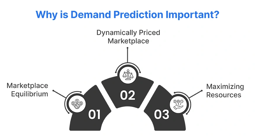
Why is Demand Prediction Important?

Here are some of the reasons why demand forecasting is so important:

• Marketplace Equilibrium: Demand prediction helps Uber establish equilibrium between drivers and riders to minimize wait times and maximize driver earnings.
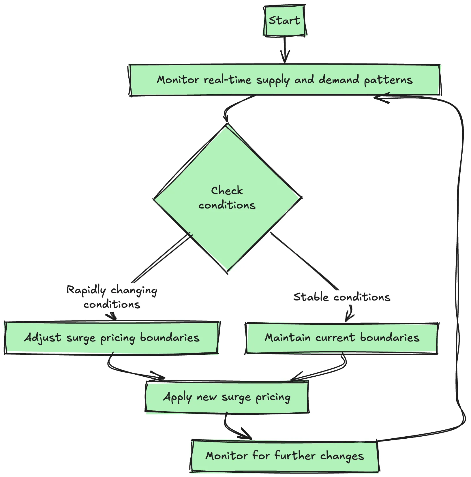
• Dynamically Priced Marketplace: Being able to accurately forecast demand enables Uber to know how many drivers they will need for surge pricing while ensuring that there are enough available during an increase in demand.
• Maximizing Resources: Demand prediction is used to inform everything from online marketing spending to incentivizing drivers to the provisioning of hardware.

Data Sources and External Signals

Uber utilizes demand-forecast models built on copious amounts of historical data and real-time signals. The history is comprised of trip logs (when, where, how many, etc.), supply measures (how many drivers are available?), and features derived from the rider and driver apps. The company considers through-the-door events as important, as real-time signals. External factors are critical, including calendars of holidays/major events, weather forecasts, worldwide and local news, disruptions to public transit, local sports games, and incoming flight arrivals, which can all impact demand.

As Uber states, “Events like New Year’s Eve only occur a couple of times a decade; thus, forecasting those demands relies on exogenous variables, weather, population growth, or marketing/incentive changes, that can significantly influence demand”.

Key Data Features

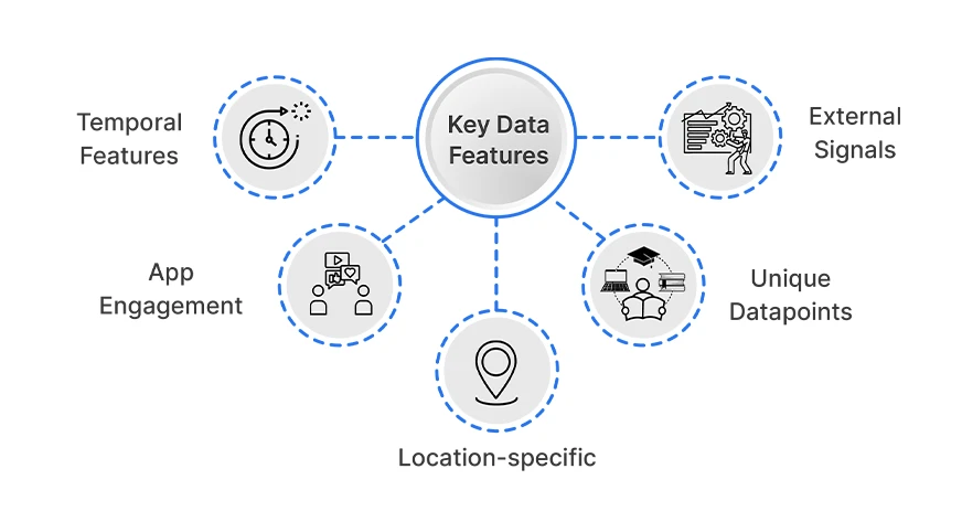
The key features of the data include:

• Temporal features: Time of day, day of the week, season (e.g., weekdays versus weekends, holidays. Uber observes daily/weekly patterns (e.g., weekend nights are busier) and holiday spikes.
• Location-specific: Historical ride counts in specific neighborhoods or grid cells, historical driver counts in specific areas. Uber is mostly forecasting demand by geographic region (using either zones or hexagonal grids) in order to assess local surges in demand.
• External Signals: weather, flight schedules, events (concerts/sports), news, or strikes at a city-wide level. For instance, to forecast airport demand, Uber is using flight arrivals and weather as its forecasting variables.
• App Engagement:  Uber’s real-time systems monitor app engagement (i.e., how many users are searching or have their app open) as a leading indicator of demand.
• Unique datapoints: active app users, new signups, which are proxies for overall platform usage.

Taken together, Uber’s models are able to learn complex patterns. An Uber engineering blog on extreme events describes taking a neural network and training it with city-level features (i.e., what trips are currently in progress, how many users are registered), along with exogenous signals (i.e., what is the weather, what are the holidays), so that it can predict large spikes.

This produces a rich feature space that is able to capture regular seasonality while accounting for irregular shocks.

Machine Learning Techniques in Practice

Uber uses a combination of classical statistics, machine learning, and deep learning to predict demand. Now, let’s perform time series analysis and regression on an Uber dataset. You can get the dataset used from here.

Step 1: Time Series Analysis

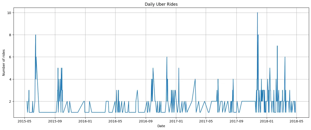
Uber utilizes time series models to develop an understanding of trends and seasonality in ride requests, analyzing historical data to map demand to specific periods. This allows the company to prepare for surges it can expect, such as a weekday rush hour or a special event.

import matplotlib.pyplot as plt

# Count rides per day

daily_rides = df.groupby('date')['trip_status'].count()

plt.figure(figsize=(16,6))

daily_rides.plot()

plt.title('Daily Uber Rides')

plt.ylabel('Number of rides')

plt.xlabel('Date')

plt.grid(True)

plt.show()

This code groups Uber trip data by date, counts the number of trips each day, and then plots these daily counts as a line graph to show ride volume trends over time.

Output:

Step 2: Regression Algorithms

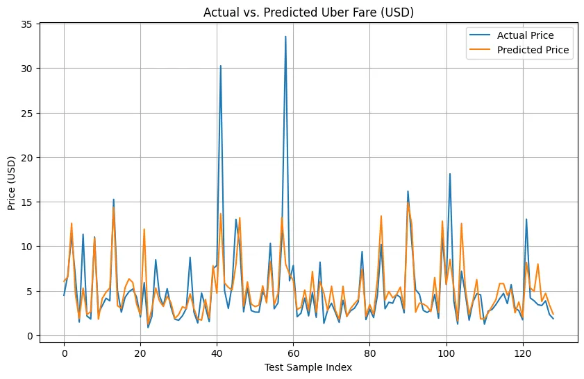
Regression analysis is another useful analytics technique that enables Uber to assess how ride demand and pricing can be influenced by various input factors, including weather, traffic, and local events. With these models, Uber can determine. 

plt.figure(figsize=(10, 6))

plt.plot(y_test.values, label="Actual Price")

plt.plot(y_pred, label="Predicted Price")

plt.title('Actual vs. Predicted Uber Fare (USD)')

plt.xlabel('Test Sample Index')

plt.ylabel('Price (USD)')

plt.legend()

plt.grid(True)

plt.show()

This code plots the actual Uber fares from your test data against the fares predicted by your model, allowing you to compare how well the model performed visually.

Output:

Step 3: Deep Learning (Neural Networks)

Uber has implemented DeepETA, basically with an artificial neural network that has been trained on a large dataset with input factors like coordinates from GPS, as well as previous ride histories and real-time traffic inputs. This lets Uber predict the timeline of an upcoming taxi ride and potential surges thanks to its algorithms that capture patterns from multiple varieties of data.

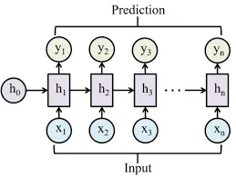
Step 4: Recurrent Neural Networks (RNNs)

RNNs are particularly useful for time series data, where they take past trends as well as real-time data and incorporate this information to predict future demand. Predicting demand is generally an ongoing process that requires real-time, effective involvement.

Step 5: Real-time data processing

Uber always captures, combines, and integrates real-time data relevant to driver location, rider requests, and traffic information into their ML models. With real-time processing, Uber can continuously give feedback into their models instead of a one-off data processing approach. These models can be instantly responsive to changing conditions and real-time information.

Step 6: Clustering algorithms

These techniques are used to establish patterns for demand at specific locations and times, helping the Uber infrastructure match overall demand with supply and predict demand spikes from the past.

Step 7: Continuous model improvement

Uber can continuously improve their models based on feedback from what actually happened.  Uber can develop an evidence-based approach, comparing demand predicted with demand that actually happened, taking into account any potential confounding factors and continuous operational changes.

You can access the full code from this colab notebook.

How does the Process work?

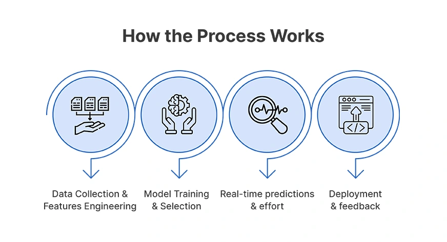
This is how this entire process works:

1. Data Collection & Features Engineering: Aggregate and clean up historical and real-time data. Engineer features like time of day, weather, and event flags.
2. Model Training & Selection: Explore multiple algorithms (statistical, ML, deep learning) to find the best one for each city or region.
3. Real-time predictions & effort: Continuously build models to consume new data to refresh forecasts. As we are dealing with uncertainty, it is important to generate both point predictions and confidence intervals.
4. Deployment & feedback: Deploy models at scale using a distributed computing framework. Refine models using actual outcomes and new data.

Challenges

Here are some of the challenges to demand prediction models:

1. Spatio-Temporal Complexity: Demand varies greatly with time and place, requiring very granular, scalable models.
2. Data Sparsity for Extreme Events: Limited data for rare events makes it difficult to model accurately.
3. External Unpredictability: Unplanned events, such as sudden changes in weather, can disrupt even the best programs.

Real-World Impact

Here are some of the effects produced by the demand prediction algorithm:

• Driver Allocation: Uber can direct the drivers to high-demand areas on the road (referred to as the fair value), send them there before the surge occurs, and reduce the drivers’ idle time while improving the service provided to the riders.
• Surge Pricing: Demand predictions are paired with demand dehydration, with automatically triggered dynamic pricing that eases the supply/demand balance while ensuring there’s always a reliable service available to riders.
• Event Forecasting: Specialized forecasts can be triggered based on large events or adverse weather that helps with resource allocation and marketing.
• Tradition of Learning: Uber’s ML systems learn from every ride and continue to fine-tune the predictions for more accurate recommendations.

Conclusion

Uber’s demand prediction is an example of modern machine learning in action – by blending historical trends, real-time data, and sophisticated algorithms, Uber not only keeps its marketplace running smoothly, but it also provides a seamless experience to riders and drivers. This commitment to predictive analytics is part of why Uber continues to lead the ride-hailing space.

Frequently Asked Questions

Data Scientist | AWS Certified Solutions Architect | AI & ML Innovator

As a Data Scientist at Analytics Vidhya, I specialize in Machine Learning, Deep Learning, and AI-driven solutions, leveraging NLP, computer vision, and cloud technologies to build scalable applications.

With a B.Tech in Computer Science (Data Science) from VIT and certifications like AWS Certified Solutions Architect and TensorFlow, my work spans Generative AI, Anomaly Detection, Fake News Detection, and Emotion Recognition. Passionate about innovation, I strive to develop intelligent systems that shape the future of AI.